Analyzing blockchain graphs with Apache Spark and Jupyter

Introduction

Cryptocurrencies attract various groups of people. Among them could be investors, people from retail, tech enthusiasts, crypto-anarchists, etc. We are not going to focus on anything other than the raw technology behind the Blockchain, leaving aside all the ideology and hype that comes with the Bitcoin.

The GraphX based notebook uses this spark-notebook as the notebook technology, while the GraphFrames based notebook uses project Jupyter. Also the second notebook connects to an existing spark cluster that was created by Oshinko tools.

Architecture

A Jupyter/Spark notebook is an interactive compute environment that interleaves documentation, code examples, and graphical output.

Similar to our other notebook examples, these notebooks are the Spark drivers that interactively send the commands to the Spark cluster for the evaluation. They can either spawn their own standalone Spark or connect to an external one.

Install and run the notebook

Installing our notebook is very simple: we just need to create an OpenShift project and install and run the notebook application. Make sure you’re logged in to OpenShift and have selected the right project, and then execute the following two commands:

oc new-app jkremser/bitcoin-notebook:tutorial-1.0.0
oc expose svc/bitcoin-notebook

for the GraphFrames notebook and the following for the GraphX notebook:

oc new-app jkremser/bitcoin-spark-notebook:tutorial-1.0.0
oc expose svc/bitcoin-spark-notebook

Once both routes are exposed, the notebooks should be available. You can find the URLs if you run oc get routes. It is also possible for the Jupyter notebook to set environment variable for connecting to an external Spark cluster.

To do that, you can optionally run this: oc new-app jkremser/bitcoin-notebook:tutorial-1.0.0 -e SPARK_MASTER=spark://c:7077

Where c is the hostname of the Spark cluster.

Usage

Both notebooks come with some prepared data in the parquet files, but part of the project is also the parquet-converter that takes the raw Blockchain data and converts it to the format that is digestible by Spark. It assumes the official bitcoin wallet to be installed that itself downloads the whole Blockchain (~150 GB). However, it works also with a partially downloaded Blockchain.

Jupyter Notebook (GraphFrames and NetworkX) This notebook is shipped by the bitcoin-notebook container and it is called blockchain.ipynb. It is the only notebook that is present in the docker image.

Interacting with the Jupyter notebook is very simple. If you select a cell with Python code you can 1) edit it or 2) execute it by pressing the "run cell" button in the toolbar or by pressing shift + enter. This notebook includes cells with instructions for running the program as well as the explanatory video about how the Blockchain internally works

The description of what the notebook actually does is be part of the notebook itself. In short this notebook demonstrates the degree distribution of the bitcoin addresses and compares with older Blockchain data. It also visualizes sub-graphs using the sigma.js library and with the NetworkX python library.
Spark Notebook (GraphX and PageRank) This notebook is called blockchain.snb.ipynb and is shipped by the container called bitcoin-spark-notebook.

While the previous notebook was looking at the graph as a whole, finding some common properties and comparing some statistics about how they developed over time, this one demonstrates the famous PageRank algorithms and finds outliers in the graph and sorts them by the significance.

It uses the Scala kernel, so while the blockchain.ipynb used Python as the programming language, this one uses Scala. This is because the GraphX can be used only from Scala, while for GraphFrames there is the Spark package available.

Expansion

Currently the number of edges in the graph is relatively large and it is due to the fact that during the conversion to parquet files we do the following: for each transaction in each block we create an edge between each input in the transaction and each output in the transaction. This means that in the case of multi-input (N), multi-output (M) transaction we end up with N times M edges.

A useful improvement would be representing the concept of a transaction in the resulting graph as a standalone node where the ingoing edges would be the inputs and outgoing edges the outputs.

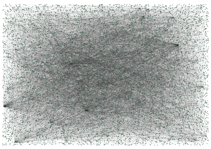
This is a visualization of 0.00005% the data.

Videos

No videos are available for this tutorial except this one from OpenSlava.